System Correction Factor SCF can customise the standard UARL equation for pipe materials, small systems and pressure: bursts relationships
Abstract
ILI – the ratio of Current Annual Real Losses (CARL) divided by Unavoidable Annual Real Losses (UARL), calculated from a leakage component analysis based on auditable parameters for well-maintained infrastructure in good condition – was developed for the 1st IWA Water Loss Task Force, chaired by Allan Lambert, and published in 1999. It was designed as a KPI for rational technical comparisons of leakage management performance between Utilities with more than around 5000 service connections and diverse system characteristics. Since then ILI and UARL have gained wide acceptance internationally, with many thousands of such calculations worldwide. A recent overview of ILIs for 212 Utility ‘whole systems’ in 4 countries with acknowledged expertise in leakage management shows median ILI values close to 1.0.
Many practitioners have since applied the UARL and ILI concept in smaller stand-alone systems, District Metered Areas and Pressure Managed Zones. In some of these small systems with low leakage (often with low managed pressures), the CARL volume calculated from an annual water balance has been less than the UARL, leading to calculated ILIs less than 1.0. This raised some questions – how can actual leakage be less than ‘unavoidable’ leakage? Does the UARL equation over-estimate CARL, and does it need to be improved for wider application in small systems with low pressures?
For systems where high ILIs identify potential for large leakage reductions, this question is not likely to be one of great urgency. However, for small systems with very low ILIs, it is important to research and identify likely causes, to be able to check for data errors and mis-assumptions in CARL and UARL calculations, and to predict more reliably ‘how low could you go’ for any size of system. Previous papers in 2009 to 2018 have identified various circumstances which could lead, singly or in combination, to calculated ILIs less than 1:
- errors in low CARL volumes derived from Water Balances, or Minimum Night Flows and Night-Day Factors
- errors in infrastructure and/or pressure data inputs to the UARL equation
- lower pressure systems where pressure: leak flow rate relationships are more sensitive than the simplified linear assumption used in the UARL equation
- systems where all bursts surface quickly or are easily and rapidly identified from night flow measurements, including small District Metered Areas.
The standard UARL equation has, over the last 20 years, proved to be both practical and robust for the great majority of Utility ‘whole systems’, and has been adopted in many countries. However, an approach for optional customising of UARL for the influences of small system size (including DMAs), diversity of pipe materials, and for the influences of pressure on burst frequency (which was not known or allowed for in 1999 UARL equation) would be useful. This paper describes how these three inter-related influences have now been combined in a new software UARL with SCF, which rapidly calculates and applies a non-dimensional System Correction Factor as a multiplier to the standard UARL equation. The SCF, which varies with pressure, takes into account specific infrastructure characteristics of any individual system, from the smallest DMA to a whole Utility
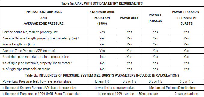
UARL with SCF has been created to allow users with small systems, low or high pressures, and different combinations of rigid and flexible pipe materials to quickly check if a customised UARL is significantly different from a standard UARL calculation. The three inter-related concepts used to calculate UARL with SCF are:
- FAVAD (Fixed and Variable Area discharges), now a widely used concept which assumes that leak flow rates vary with average zone pressure to the power 0.5 for bursts on rigid pipes, and with pressure to the power 1.5 for bursts on flexible pipes and for small undetectable ‘background’ leakage at joints and fittings.
- Use of Median UARL burst numbers: bursts in small systems are rare events with positively skewed probability distributions. The median value lies at the mid-point (50%ile) of a series of annual burst numbers, with equal probability of falling above or below it. It is a more robust and ‘typical’ value than the mean. As burst numbers increase in larger systems, the Median closely resembles the Normal (Gaussian) bell- shaped probability distributions, where Mean and Median (the middle value in a series and of annual burst numbers) are the same.
- Pressure: burst frequency relationships for mains and services, which were not known or included in the standard UARL equation in 1999, but have since been researched and quantified, and applied internationally since 2013.
1. Brief Review of the Standard UARL Equation (Metric Version)
Auditable assumptions used to derive coefficients in the UARL equation (Figure 1) were originally agreed by the 1st IWA Water Loss Task Force (Lambert et al, 1999) as being appropriate for application to historically grown, large, well-managed Utility distribution systems with mixed pipe materials. The abbreviated terms Lm (for mains length), Nc (for number of service connections, main to property line) and Lp (for underground supply pipe length) will be used as abbreviations for infrastructure components in this paper.
Figure 1: The 1999 UARL Equation (metric units)
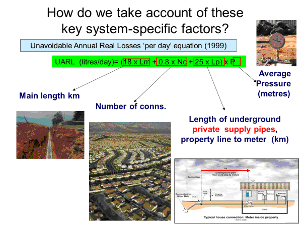
Acknowledgement: Liemberger
Versions of the standard UARL equation in other units of flow, mains and pipe length and pressure are available, see https://www.leakssuitelibrary.com/uarl-and-ili/ .
Several circumstances in which the standard UARL formula may be expected to overestimate annual real losses volume were summarised in a study of Austrian OVGW data from small systems by Lambert, Koelbl and Fuchs-Hanusch (2014) as:
- systems where very few leaks are unreported due to ground conditions
- small systems where continuous night flow identifies leaks soon after they occur
- small relatively new systems with lower frequency of bursts on mains and service connections than the frequencies assumed in the standard UARL equation
- more sensitive pressure:leak flow relationships for mains and services with flexible pipe materials at pressures significantly lower than 50 metres
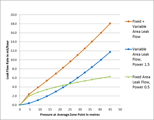
Flow rates from Fixed Area leaks on rigid pipes (ring cracks, corrosion holes, blowouts) are less sensitive to changes in pressure, but flow rates from Variable Area leaks (where leak area changes linearly with pressure) are more sensitive to changes in pressure. Background (undetectable) small leaks at joints and fittings are also Variable Area leaks. Different combinations of Fixed and Variable Area leaks for mixed pipe materials in larger systems may often result (Figure 2) in an approximately linear pressure:leak flow rate relationship (as used in the standard UARL equation), but pipe materials in smaller systems can vary widely, from 100% rigid to 100% flexible.
Figure 2. Fixed and Variable Area Leak Flow Rate vs Average Zone Pressure
Key parameters in the UARL standard equation shown in Table 1 were based on international data at 50 metres pressure using auditable assumptions.
Table 1: Parameter Values for Bursts Frequency in UARL Standard Equation
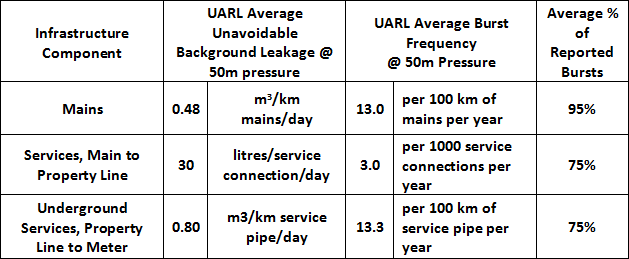
Source: Lambert 2020
The UARL is based on component analysis of different types of leaks, with different frequencies, typical durations and flow rates. The largest component of UARL (usually 60% to 70%) is unavoidable (and undetectable) background leakage; reported and unreported bursts typically account for the remaining 30% to 40% of UARL volume.
2. Customising the UARL Equation for Lower and Higher Pressures, based on Pipe Materials and FAVAD
In the absence, in 1999, of any known relationship between pressure and burst frequencies (on mains, and on services) the UARL average burst frequencies at 50 metres pressure shown in Table 1 were assumed to apply at all other pressures. This aspect has now been included in the SCF approach, as explained in Part 4 of this paper.
Also in 1999, the simplified linear (power 1.0) average pressure correction for all leak flow rates in Figure 2 was used for systems with lower or higher pressure than 50 metres. However, by 2005 it had been recognised that in some circumstances the assumed linear pressure:leak flow relationship could over-predict UARL at lower pressures in systems with high proportions of ‘variable area’ leakage paths from background leaks and flexible pipe materials. Figure 3 shows a Pressure Correction Factor (PCF) that could be applied as an optional multiplier to the UARL equation for systems with different overall proportions of rigid pipes, from 100% rigid/0% flexible to 0% rigid/100% flexible. An intermediate curve, for 50% rigid/50% flexible pipe materials (calculated as a simple overall % for mains and services together in this graph) is also shown.
Figure 3: Influence of type of pipe materials on UARL as pressure changes
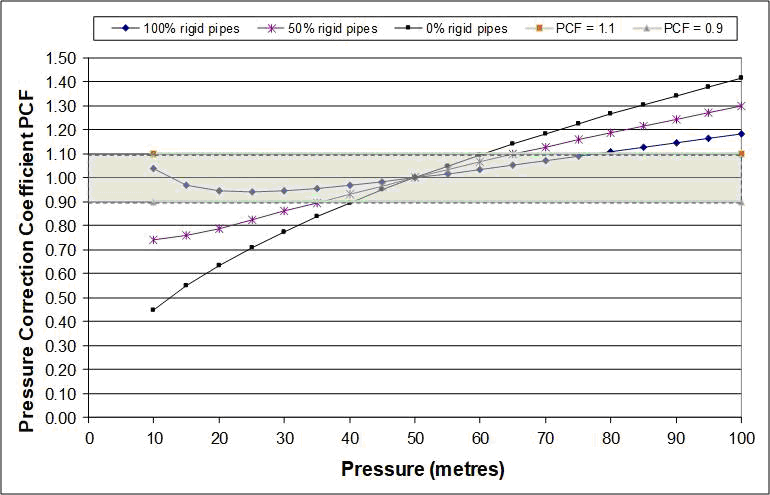
Source: Lambert, IWA Water Loss, Cape Town, 2009
For the purpose of this calculation:
- rigid pipe materials include Cast/Ductile/Galvanised Iron, Copper, Concrete, Fibre-cement, lead and other materials where the area of individual bursts does not vary significantly with pressure.
- flexible pipe materials include MDPE, HDPE, Polyethylene, uPVC and other materials where the area of individual background leaks and bursts expands and contracts with changes in pressure.
When Figure 3 was published in 2009 in a 10-year review of use of UARL, it was accompanied by a relaxation of limits of application of the UARL Equation as shown in Table 2, as several experienced leakage consultants considered the UARL calculation to be very useful in Low and Middle Income Countries for low pressure systems with high leakage and fewer than 3000 service connections, even though the standard UARL equation would lead to over-estimates of the true UARL.
Table 2: Relaxation of limits of application of UARL Equation, 1999 to 2009 (superceded in 2020)
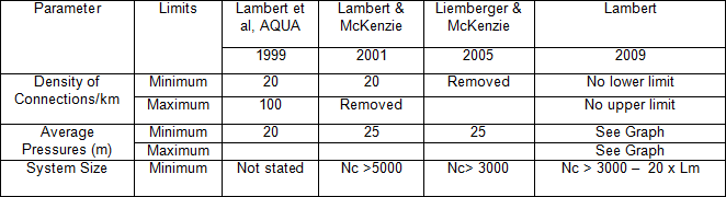
Source: Lambert, 2009
However, care was obviously needed in situations where the Standard UARL equation would consistently over-estimate and lead to ILIs less than 1.0. As pressure management to reduce both leak flow rates and bursts became increasingly used internationally after 2009, ILIs less than 1 were more frequently reported in some High-Income Countries in which a large percentage of all Utilities were small systems.
The UARL with SCF new approach now permits direct rapid calculation of a customised graph and Table (UARL with FAVAD option) for an individual system with any specified % rigid: % flexible pipes in each section of infrastructure – Lm, Nc and Lp (if the meter is not located close to property line). This is an optional discretionary improvement if the person doing the UARL calculation considers that the standard UARL formula may need to be customised only for pipe materials, particularly for systems with significant percentages of flexible pipe materials, at average pressures significantly lower than 40 metres or higher than 60 metres, as indicated in Figure 3.
3. Analysis of Low Burst numbers in Small Systems, using the Poisson Probability Distribution
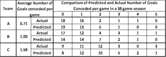
The Poisson probability distribution can be used for modelling the number of times an event occurs in an interval of time or space. It can be used to predict the probabilities of occurrence of numbers of isolated events, when only the average number over several periods in a continuum of time is known. A commonly quoted example of using a Poisson distribution is to predict how often a football team is likely to concede 0, 1, 2, 3 etc goals per game in a season, knowing only the average goals per game over a full season. In Table 3 below, the number of times goals were conceded as predicted by the Poisson distribution for 3 teams in the English Premier League in a 38 game season compare well with the actual number of games and goals conceded.
This example is shown to demonstrate a practical use of a Poisson distribution, for readers who may be put off by its somewhat intimidating mathematics (which can be found on Wikipedia).
Table 3: Goals per football game in English Premier League: Actual and Predicted
These figures are originally derived as probabilities, and the methodology has been used by the author to model the probability of 0, 1, 2, 3 etc bursts for different size distribution systems, based on annual average UARL burst frequencies from Table 1.
Figure 4 shows the Poisson probability distributions for average UARL burst frequencies of 1, 2, 3 … 15 bursts per year. Some corresponding infrastructure parameters in terms of Number of Connections (Nc) and km of mains Lm) are shown on the upper horizontal axis for comparison.
Figure 4: Poisson Distributions for Annual Average UARL Burst Numbers at 50 metres pressure, linked to Infrastructure Parameters
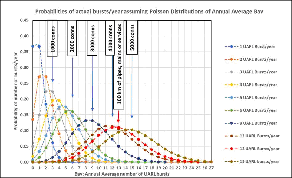
Source: Lambert 2019
As number of service connections progressively reduces below 5000, the probability distribution becomes increasingly skewed, with a higher probability of lower numbers of bursts. For example, at an expected UARL average of 1 service burst per year at 50 metres pressure (for 333 service connections), there is a 37% chance of no bursts, a 37% chance of 1 burst, an 18% chance of 2 bursts, and a 6% chance of 3 bursts. So when the standard UARL equation with average burst frequencies is used, it will over-predict the UARL burst numbers.
Small systems will have many different combinations of Lm, Nc, and Lp (which is zero if the meter is located at or very near the property line). Also, reported and unreported bursts on mains and services have different typical average flow rates at 50 metres pressure, and unreported bursts run for longer and individually lose a greater volume of water than reported bursts – around 8 times as much for unreported mains bursts, and 12 times as much for unreported service connection bursts.
It is therefore necessary to calculate separate probability distributions of number of reported and unreported bursts for each of the 3 components of infrastructure Lm, Nc, Lp in the UARL equation, and to derive equations which can be used to calculate median numbers of up to 6 components of UARL bursts at 50 metres pressure for any combination of values of Lm, Nc and Lp.
The SCF for FAVAD plus POISSON option permits direct rapid calculation of customised graphs and Tables for an individual system with any specified % rigid: % flexible pipes in each section of infrastructure – Lm, Nc and Lp – assuming that the median of the original 1999 UARL burst frequencies varies with system size but not with pressure.
This is a discretionary option if the person doing the UARL calculation considers that the standard UARL formula may need to be customised for small system size in addition to the effects of FAVAD on pipe materials, but wishes to continue to assume that the 1999 original UARL average burst frequencies at 50 metres pressure are used, whatever the actual average pressure. The Poisson probability distribution is skewed for very small systems, but also closely represents a normal distribution when number of service connections increases above around 5000 service connections, so the SCF for FAVAD + POISSON can also be applied to larger systems. The complexity and large number of these calculations required a specialist software UARL with SCF which was developed in metric and US version units by Water Loss Research and Analysis Ltd, originally for research purposes during 2019.
4. Customising the UARL Equation for Pressure:Bursts Frequency Relationships
In 1999, there was a growing awareness that reduction of maximum pressures could reduce burst frequency, but this suggestion was not generally accepted due to shortage of documented international evidence. The burst frequencies used in the original UARL standard equation for around 50 metres pressure were therefore assumed to apply over all typical ranges of distribution system pressures, as no commonly agreed relationship between pressure and burst frequency existed at that time.
From 2003 onwards, ‘before’ and ‘after’ bursts data from numerous pressure management schemes collected by members of the IWA Water Loss Task Force clearly proved such relationships did exist, and they have since been increasingly documented, quantified, researched, improved, tested and applied internationally. The general pressure: burst frequency relationship option now used to calculate SCF with FAVAD, POISSON and PRESSURE: BURSTS was originally developed by the author in the period 2011 to 2013, using data from multiple pressure management schemes implemented in Australian Utilities in 2009 to 2011 during the Millenium Drought. It has since been tested and successfully used to prioritise and predict burst reductions in Zones in large Utilities in South Africa, England and Wales and elsewhere. The author considers that now is an appropriate time to include this pressure: bursts relationship as a 3rd concept in an optional calculation in the UARL with SCF software.
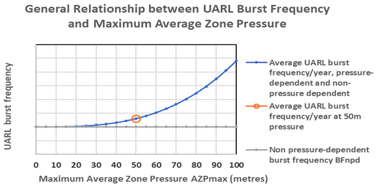
The general form of relationship to be used for each infrastructure component is shown in Figure 5, and consists of two components, which when added together at 50 metres pressure equals the 1999 UARL average burst frequency.
- BFNPD: a ‘non-pressure-dependent burst frequency’ derived from sample data for infrastructure in good condition in high-income countries
- BFPD: a pressure-dependent component which varies with the maximum value of the Average Zone Pressure cubed
UARL with SCF software is designed to permit future changes in these assumptions if they should prove more appropriate at some future date.
Figure 5: Pressure: Burst Frequency Relationship assumed in UARL with SCF
The SCF with FAVAD plus POISSON + PRESSURE: BURSTS permits direct rapid calculation of customised graphs and Tables for an individual distribution system with any specified % rigid: % flexible pipes in each section of infrastructure – Lm, Nc and Lp – using the median values of the original 1999 UARL burst frequencies, varying with system size and Average Zone Pressure.
The effect of this additional Pressure:Bursts correction to the SCF for FAVAD + POISSON + PRESSURE:BURSTS is to quite rapidly increase UARL burst frequencies and SCF at pressures greater than 50 metres, and slightly reduce UARL burst frequencies as pressure reduces below 50 metres.
The Poisson probability distribution is skewed for very small systems, but also closely represents a normal distribution when number of service connections increases above around 5000 service connections, so SCF for FAVAD + POISSON + PRESSURE:BURSTS can also be applied to larger systems.
Following numerous calculations using this software, in 2020, the table summarising limits of application of the UARL equation was updated as follows:
Table 4: Updated limits of application of UARL Equation, 1999 to 2020
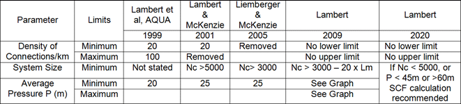
Source; Lambert 2020
Two screenshots of the UARL with SCF software are shown in Appendix 1, for a system with 5000 service connections and a sub-system with 1000 service connections having the same pressure, and the same proportional infrastructure.
Summary
The UARL with SCF software can be used to rapidly calculate a customised System Correction Factor for any Zone or System, then applied as a multiple to the standard 1999 UARL equation.
In the SCF with FAVAD option, the Fixed and Variable Area concepts of pressure:leak flow relationships are applied separately to 3 components of infrastructure (mains, and the two sections of the service connection split at the property line), using different %s of rigid and flexible pipes for each infrastructure component.
In the SCF with FAVAD and POISSON option, the Fixed and Variable Area concepts of pressure:leak flow relationships are applied, and the average UARL burst numbers are converted to Median (50% exceedance) burst numbers for the specific infrastructure parameters in the system under review. The original (1999) average UARL burst frequencies at 50m pressure are used for all calculations.
In the SCF with FAVAD, POISSON and PRESSURE:BURSTS, the average UARL burst numbers are adjusted for pressure:bursts before calculating the Median burst numbers for the system under review, and the Fixed and Variable Area concepts of pressure:leak flow relationships are then applied. The average UARL burst numbers are then converted to Median (50% exceedance) burst numbers for the specific infrastructure parameters in the system under review.
In all cases, the calculated SCF at the chosen Average Zone Pressure for the three options listed above is shown as a Table, followed by a Table of Standard UARL and UARL for each of the 3 SCF sets of options in volume/day. A bar chart compares the burst frequencies of each of the 3 SCF sets of options. There is a graph and Tables of SCF vs pressure for each of the 3 sets of options; and a graph and Table of UARL in volume/day vs pressure for each of the 3 sets of options, compared with Unavoidable Background Leakage, for pressures between 10 and 100 meters pressure.
Users can then decide if it is appropriate to apply an SCF, based on whether the standard UARL equation is sufficiently reliable for their purposes, or not.
This research adds to our general understanding of why some small systems can achieve real losses in some years which are less than the UARL predicted by the 1999 standard UARL equation.
The UARL with SCF software is now being provided by WLR&A Ltd as a service to international Utilities and Consultants wishing to derive more generalised relationships between SCF and Lm, Nc and Lp, taking account of pressure, connection density and other system parameters.
It is expected that UARL with SCF will be particularly useful to
- identify individual Zones in which achievable median UARL volumes are smaller than volumes derived from the standard UARL equation
- identify systems at pressures in excess of 50 metres in which achievable median UARL volumes are higher than volumes derived from the standard UARL equation
- demonstrate how reduction of excess average pressure will reduce the median UARL to a greater extent than was assumed by the standard UARL
The data entry requirements and assumptions for each of the 4 options for calculating UARL are summarised in Tables 5a and 5b.
Acknowledgements
To John May (deceased) for his inspirational insights into pressure:leakage relationships and pressure:bursts relationships 25 years ago.
To Codingdale Ltd for developing the online UARL for SCF software to WLRandA Ltd specifications. The Copyright for UARL with SCF software is held by WLRandA Ltd.
Software: Additional information on UARL with SCF software in metric and US Units can be found at https://www.wlranda.com/software/
Appendix 1: Two Examples showing influence of Pipe Materials, Small System size and Pressure
Figure A1 summarises the UARL with SCF calculation for a distribution system (Example 1) with:
- 5000 service connections, main to property line, with 20% rigid and 80% flexible pipe materials,
- Customer meters located on average 10 metres after the property line (50 km total length) with 50% rigid and 50% flexible pipe materials
- 125 km of mains, with 80% rigid and 20% flexible pipe materials
- Density of connections 40 per km mains
- Average Pressure 35 metres
Figure A1: 5000 service connections, 10m/connection property line to meter, 125 km mains
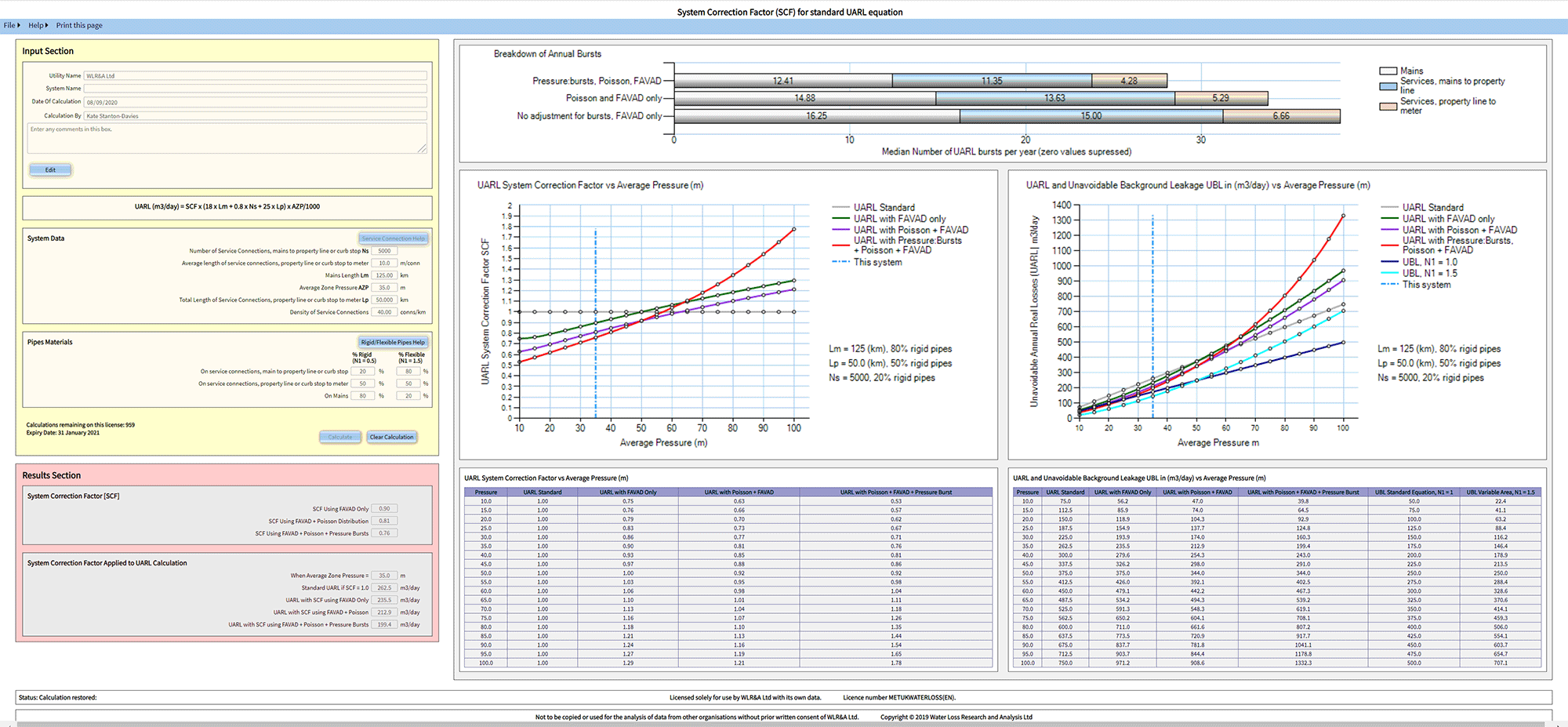
© Water Loss Research and Analysis Ltd, reproduced with permission.
The 7 items of Data entry are shown in the yellow section. Calculated SCFs, and standard and modified UARLs in volume/day at 35 metres pressure, are listed in the pink section. The two central graphs and the two tables below them show how the calculated SCFs and the UARL volumes per day are predicted to vary with average pressure (unavoidable background leakage is also shown).
The calculated reductions in UARL burst numbers on each of the 3 infrastructure components at 35 metres pressure is shown in the upper horizontal bar chart.
Depending upon which assumptions are made (Standard UARL, FAVAD only, FAVAD and Poisson, or FAVAD, Poisson and Pressure:Bursts), the right hand graph and Table in volume/day can be used to interpret the increase or decrease in UARL per metre of pressure, if pressures are reduced (or allowed to rise). In this example, at 35 metres pressure, it is 8 m3/day for 1 metre of pressure.
Each distribution system, zone or DMA will have its own signature characteristic curves for SCF vs average pressure, and for UARL in volume per day vs average pressure.
Figure A2 summarises the UARL with SCF calculation for Example 2, a distribution system one-fifth of the size of Figure A1 (1000 services, 25 km of mains) with the same proportional dimensions (40 connections per km), infrastructure characteristics, %s of rigid pipes and average pressure of 35 metres.
Figure A2: 1000 service connections, 10m/connection property line to meter, 25 km mains
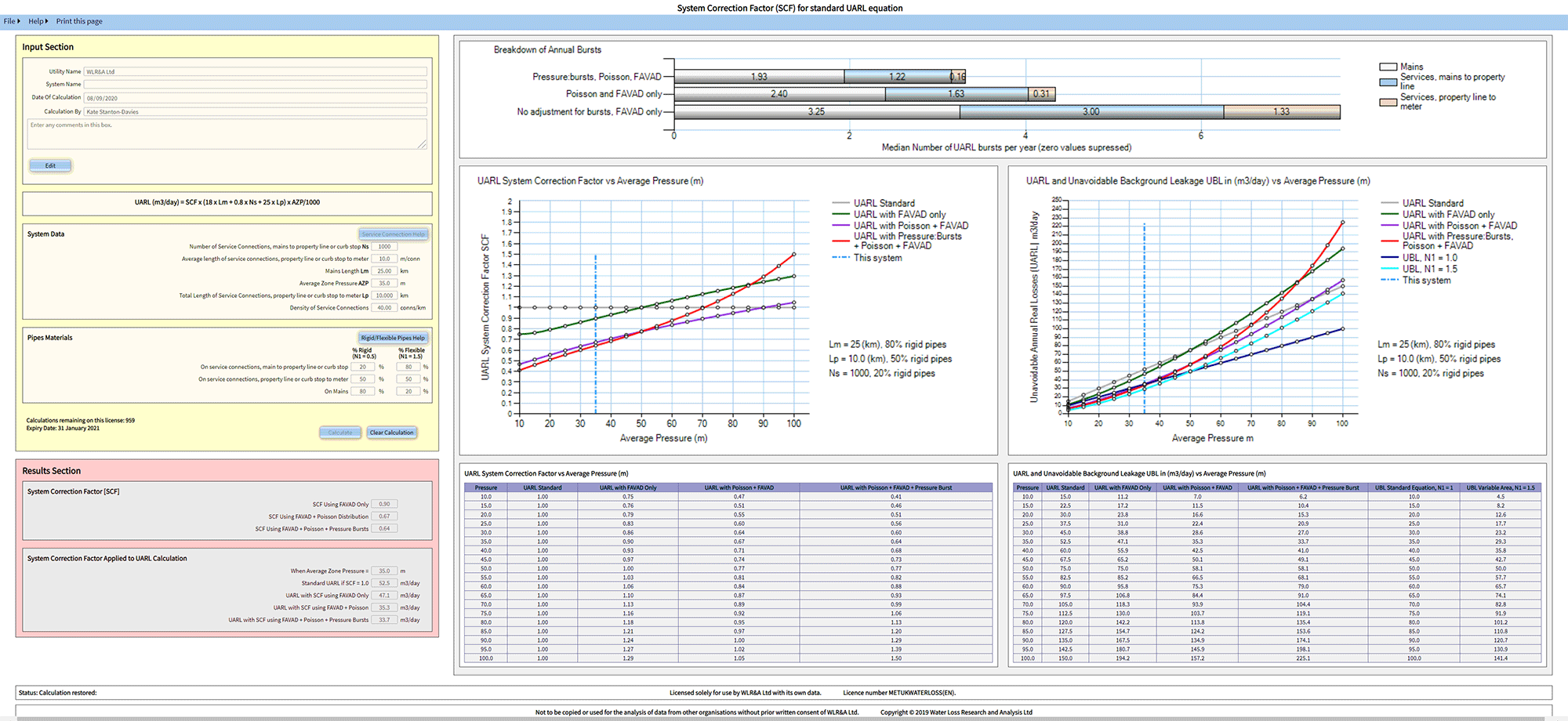
© Water Loss Research and Analysis Ltd, reproduced with permission.
The proportional reduction in UARL bursts is up to 57% in the smaller system, but only up to 26% in the larger system, showing how the combination of pressure:burst frequency relationships and Poisson probability distributions are likely to progressively influence median UARL burst numbers in very small systems as system size decreases.
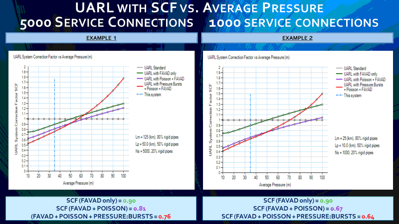
Figure A3 compares the SCF vs average pressure curves for Example 1 (5000 services) and Example 2 (1000 services).
The green curves (FAVAD only) which do not take account of Poisson or pressure:bursts relationships are the same, and predict how this particular combination of pipe materials is expected to influence how the UARL leak flow rates (including background leakage) will vary with pressure. The SCF at 35 metres pressure is 0.90 in both cases.
Figure A3: Comparisons of SCFs vs Average Pressure for 5000 and 1000 service connections
© Water Loss Research and Analysis Ltd, reproduced with permission.
Comparison of the blue curves (FAVAD + Poisson) shows how use of a Poisson (rather than a ‘Normal’) probability distribution to calculate median UARL bursts has a bigger influence as system size decreases below 5000 service connections. The SCF reduces from 0.90 to 0.81 for the larger system, but from 0.90 to 0.67 for the smaller system.
Comparison of the red curves (FAVAD + Poisson + Pressure:Bursts) shows:
- Further reduction of SCF at pressures less than 50 metres (e.g. at 35 metres, 0.81 to 0.76 for the larger system, and 0.67 to 0.64 for the smaller system)
- Larger increases in SCF at pressures more than 50 metres (e.g. at 70 metres, 0.76 to 1.18 for the larger system, and 0.64 to 0.99 for the smaller system).
These are just two examples from an almost infinite number of possible combinations of infrastructure statistics Ns, Lp, Lm, % rigid pipe materials for Ns, Lp, Lm, and average pressure. However, an appropriately designed (and admittedly complex) software allows individual calculations to be completed in a few minutes. As infrastructure lengths and materials for any particular system, Zone or DMA usually change quite gradually over time, one calculation for a range of pressures should be reasonably valid for a number of years.
The author is continuing to use this new and powerful tool to investigate interactions between system size, infrastructure dimensions, pipe materials, burst frequencies and pressure.